Modulef
Next: 2.4 Three-dimensional meshes REFEXX Up: 2 Visualization of meshes Prev: 2.2 Two-dimensional meshes TRNOXX Contents

2.3 Three-dimensional meshes TRNOXX

2.3.1 Aims and utilization limitations

Preprocessor TRNOXX is used to visualize meshes (the 3D case is described here). It is also used, for an elasticity problem for which the displacements are known, to visualize the deformed mesh (the displacements, multiplied by a given factor, are added to the nodes of the initial mesh).

Note:

The visualization of deformations are only possible in the following cases:

the finite elements are of type Lagrange,
the displacements are the NDIM (3 here) first degrees of freedom of each node,
where ND is the number of degrees of freedom per node.

For other cases, preprocessor TRC3XX, strictly requiring data structures MAIL and COOR, is used.

2.3.2 Utilization of TRNOXX (3D)

Activate preprocessor TRNOXX.
Choose the output terminal.
Input the name of the file containing the mesh.
The general menu is displayed (see further down).
Type 0 to obtain an automatic plot.
To obtain the values of the visualization parameters, type V.
Modify these values, if necessary, by choosing the corresponding key and entering the required information. Once the desired state is obtained, type 0 to display the plot.
A graphics menu is displayed on the plot to perform modifications, to exit or to return to the menu mentioned above and described in the coming sections.

2.3.3 Complete description of TRNOXX (3D)

The first part of this description presents the different notions necessary for a thorough understanding of the operations performed when visual-ising a three-dimensional mesh.

Observation conditions:

The module automatically calculates the extrema corresponding to the mesh under consideration, which are used to define the corners of the box in which the plot is displayed.

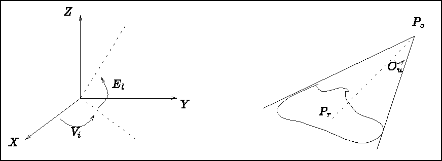
The observation conditions of a three-dimensional mesh are defined by:

the barycentre of the box defined above, which is the point viewed,
the observation point, , which is calculated in such a way that the entire object is viewed with a span , an observation angle (or longitude) and an elevation (or latitude) . In practice, fixing , and degrees, the distance is calculated such that the object is viewed in full.

Figure 2.6: Observation mode

Note that the observation angle and point are such that the extrema are taken vis-a-vis this point which, a priori, defines extrema which are different to those of the initial box, as shown in figure 2.7 which is reduced to the 2D case for an improved readability (the natural extrema M and m are replaced by the couples or depending on the choice of or ).

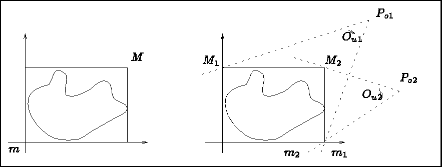
Figure 2.7: Extrema function of the observer

Automatic mode corresponds to the above specified choices for the values of , and . In manual mode, the user specifies:

the observation angle, the elevation and the span ( and ), or
the points and (in Cartesian coordinates).

The type of observation mode and the corresponding parameters are displayed in the menu (key 15 and 16, or key 15, 17 and 18). Once the plot is displayed, the two sets of parameters are indicated and the user can easily change from one observation mode to another.

Visibility:

In dimension 3, the readability of a plot depends very much on the manner in which is plotted. There are, a priori several types of plots:

a solid line plot of the edges and elements,
plots taking into account the visibility of items in the mesh which includes algorithms of the hidden parts.

The notion of visibility is interpreted differently depending to the capabilities of the computer terminal used. For a terminal without selective deletion, an edge is called visible if the normal of the face to which it belongs is directed towards the observation point . This simple algorithm presents some imperfections. For more advanced terminals, it is replaced by a a "painter" type algorithm : the faces are sorted and then plotted by starting by those furthest off, so that only those faces that are not hidden by the closer up faces are visible on the plot.

Choice of items to display:

A three-dimensional mesh can be displayed by plotting:

all the elements in solid line mode, shrunken or not,
the outer surface only by plotting its faces, generated by displaying:
- all the edges with or without elimination (by default) of edges belonging to two adjacent and coplanar faces. Two faces are called coplanar if their normals are identical w.r.t. a coefficient (by default 0.00001, value modified via key 53 (see below)).
- all the visible edges with or without this elimination.
- all the hidden edges with or without this elimination.

The faces can be colored-in, or not.

The general menu of TRGEOM (module called in this case) is given below.

 ------------------------------------------------------------
 | 10 | PLOT TYPE                 |         MESH ONLY
 ------------------------------------------------------------
 | 11 | DEVICE NUMBER             |              1
 ------------------------------------------------------------
 | 20 | MESH TO PLOT              |         c3.nopoi
 ------------------------------------------------------------
 | 15 | OBSERVATION MODE          | LONGITUDE / OX  LATITUDE  APERTURE
 ------------------------------------------------------------
 | 16 | LONGIT. LATIT.  APERTURE  | 30.00000  30.00000       10.00000
 ------------------------------------------------------------
 | 31 | QUESTIONS ABOUT THIS MESH |          NO
 ------------------------------------------------------------
 | 30 | PLOT SIZE                 |         AUTO
 ------------------------------------------------------------
 | 40 | CHARACTER TYPE            |         HARD
 ------------------------------------------------------------
 | 50 | ITEMS TO BE PLOTTED       | EDGES OF OUTER SURFACE (ALL)
 ------------------------------------------------------------
 | 51 | COPLANAR EDGES            |         ELIMINATED
 ------------------------------------------------------------
 | 53 | COPLANARITY CRITERION     |           0.1000000E-04
 ------------------------------------------------------------
 | 54 | COLOUR-IN FACES           |         COLOURED-IN FACES
 ------------------------------------------------------------
 | 56 | FACE ORIENTATION          |         ORIENTED
 ------------------------------------------------------------
 | 88 | STEREO VISION             |          NO
 ------------------------------------------------------------
 | 60 | LEGEND                    |         YES
 ------------------------------------------------------------
 | 70 | NUMBER                    |         NONE
 ------------------------------------------------------------
 | 80 | LINE TYPE                 |         SOLID
 ------------------------------------------------------------

A default value is proposed for each option. The above table lists the choices made automatically. To obtain the corresponding plot, type 0.

A key (number) and status corresponds to each item. To modify the status, it suffices to type the key and enter (see general introduction) the values corresponding to the desired state. Some options are identical to those used for two-dimensional meshes and have therefore already been described, and will thus be mentioned briefly only.

Key 10:

the plot type: mesh only (default choice), we can also request to visualize a mesh and its deformation: type 10 after which the program requests the name of the file containing data structure B of displacements. A number of additional lines then appears on the general menu (see below).

Key 11:

the device number.

Key 20:

the name of the file containing the mesh. To change files, we activate this key and input the new file name.

Key 15:

the observation mode: longitude and latitude (default mode). By typing 15, we go from one mode to the other (viewed point, observation point) whose parameters are accessible via key 17 and 18.

Key 16:

the observation conditions, i.e. the values of

and

(by default 30, 30 and 10 degrees respectively). To modify these values, type the key number and enter the new values.

Key 31:

by activating this key, we can make inquiries about the mesh and obtain information regarding its contents.

Key 30:

the plot will be full screen, otherwise the user must specify the size in cm.

Key 40:

the type of characters plotted: hardware (by default), software if not.

Key 50:

the choice of items to plot: the triangulation (by default). By activating this key, we have a choice between:

  -- INITIAL MESH                                 :
     NOTHING (CHECK ONLY)      : 0
  ** OUTER SURFACE EDGES (ALL) : 1
     OUTER SURFACE EDGES (VIS.): 2
     SURFACE EDGES (INVIS.)    : 3
     SHRINKED SURFACE (ALL F.) : 4
     SHRINKED SURFACE (SEEN F.): 5
     SHRINKED SURFACE (HIDDEN F.): 6
  ** ALL ELEMENTS              : 7
     ALL SHRINKED ELEMENTS     : 8 ?

Key 51:

only the edges not belonging to two adjacent faces, coplanar (by default) w.r.t. the coefficient contained in key 53, are not plotted. By typing 51, all edges are plotted.

Key 53:

the coplanarity coefficient (0.00001 by default), by typing this key the default value can be modified.

Key 54:

the faces are colored-in (yes, by default), type 54, to obtain the inverse choice.

Key 56:

orientation of the faces (yes, by default). This signifies that during the elimination of the hidden faces, we only plot the faces facing the observer. By selecting this key, the opposite state is obtained.

Key 88:

stereoscopy (no, by default), yes by typing 88 (if the terminal allows it).

Key 60:

the general legend (there is a legend by default) corresponds to the indications appearing to the right of the plot (see examples: title, date, file name, ...). By typing 60, we specify that we do not want the general legend.

Key 70:

the numbers to be displayed, none (by default) or, by activating this key, the choice between:

    NO NUMBER          : 0
    ELEMENT : 1 - POINT: 2 - NODE  : 3
    SUB-DOMAIN         : 4
    REFERENCE (ALL)    : 5
    REFERENCE POINTS   : 6 - NODES : 7
    REFERENCE EDGES    : 8 - FACES : 9

Key 80:

the type plot desired: solid (by default) or, by activating this key, the choice between:

    SOLID      : 1  --   DOTTED    : 2
    DASHED     : 3  --   MIXED     : 4 ?

Once a plot is displayed on the screen, a graphics menu appears which allows us to:

Exit (0) from the session,
Continue (1), i.e., return to the module's main menu;
Display the next (2) or previous (3) view;
Refresh (4) the screen;
Zoom (5);
Define a section (6) (action described below),
Move the observer to the right (R) , the left (L) , the top (T) , the bottom (B), closer (+), further (-),
Produce a hardcopy (9) of the screen, or a softcopy (8) on another graphical terminal; having done this, the user is returned to the initial state (of this graphics menu).

All these options are identical to those seen in the two-dimensional case. Only the section is specific. and , the observation and view points remaining unchanged, we enter the sides of the two planes which is used to limit the part of the object to be displayed (by default the two sections are positioned at 0. and , which corresponds to viewing the entire object).

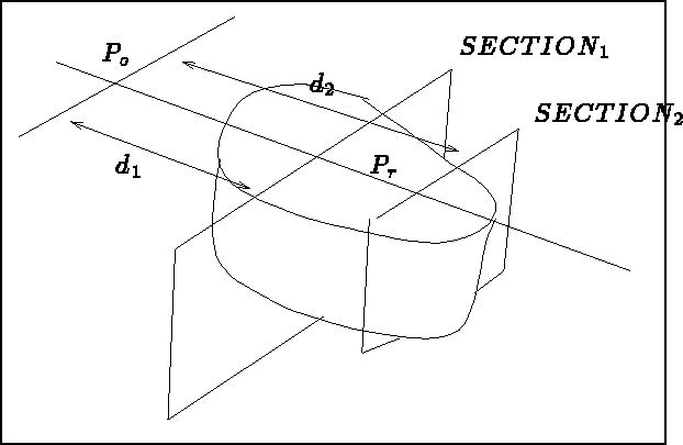
Figure 2.8: Definition of the two extremal sections

Mesh and deformation:

The module (see utilization limitations) enables us to visualize a mesh and its deformed state. The deformed mesh is obtained by adding (with an amplification factor) the calculated displacements to the nodal coordinates.

For those cases possible, the selection of key 10 results in a general menu which is identical to that of TRNOXX for the two-dimensional case, to which the reader is referred.

Examples:

Some examples of plots of three-dimensional meshes, obtained via TRNOXX, are shown in figures 2.9 to 2.13. Note that the graphics menu does not appear as the figures correspond to a softcopy performed on a laser printer, and as this terminal does not have any input possibilities.

The plots were obtained by typing the following sequences:

figure 2.9 : -1 crochet.nopo 0 8 2 bw ncadre nlogo x12 y12 fcrochet1 v
figure 2.10 : (starting with the above) 1 50 2 51 0 D 8 2 bw ncadre nlogo x12 y12 fcrochet2 v
figure 2.11 : -1 levier.nopo 50 7 0 8 2 bw ncadre nlogo x12 y12 flevier1 v
figure 2.12 : (starting with the above) 1 50 5 54 0 H 8 2 bw ncadre nlogo x12 y12 flevier2 v
figure 2.13 : -1 euclid.nopo 50 2 0 5 5 8 2 bw ncadre nlogo x12 y12 feuclid1 v

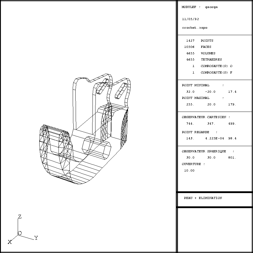
Figure 2.9: Example TRNOXX 3D: automatic mode

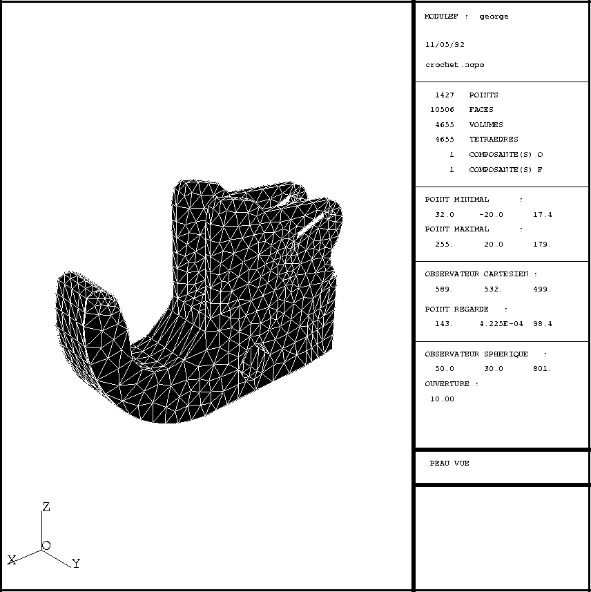
Figure 2.10: Example TRNOXX 3D: outer surface viewed without elimination

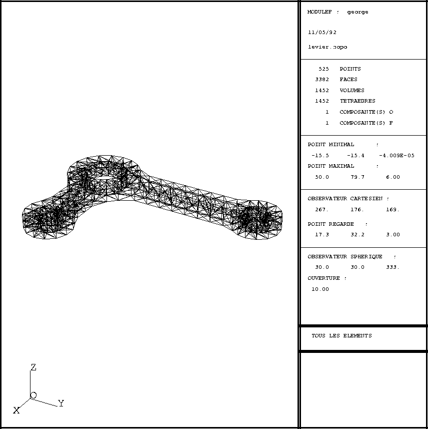
Figure 2.11: Example TRNOXX 3D: solid line plot

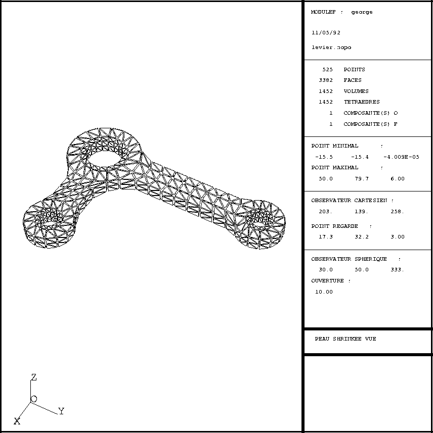
Figure 2.12: Example TRNOXX 3D: displacement and shrunken faces

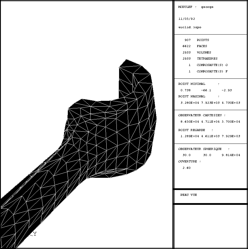
Figure 2.13: Example TRNOXX 3D: faces viewed and zoom

Next: 2.4 Three-dimensional meshes REFEXX Up: 2 Visualization of meshes Prev: 2.2 Two-dimensional meshes TRNOXX Contents