Next: 2 Conversational tests Up: 1 Introduction Prev: 1 Introduction Contents
![]()
![]()
![]()
![]()
![]()
![]()
![]()
![]()
Next: 2 Conversational tests
Up: 1 Introduction
Prev: 1 Introduction
Contents
The following simple example enables us to illustrate how to solve a problem with the help of MODULEF. This also gives us the opportunity to introduce the finite element notation used.
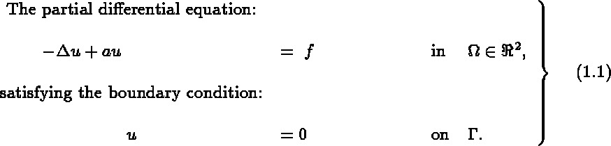
We start by formulating the boundary value problem, from which the variational formulation is derived. The finite element approximations and computer implementation are then discussed briefly, describing the various steps to be executed to solve the problem numerically using the modules in the MODULEF library. To achieve this, let us consider the Dirichlet problem described below:
Consider the following Dirichlet boundary value problem:
where
 , and
, and
 , i.e.,
 , where
  is a regular open subset of
  with a regular boundary
  .
.
The variational (weak) formulation derived from the boundary value problem is given by:
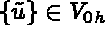
Find  , the space of admissible functions, such that
for all  .
.
The variational formulation of the problem is the point of departure for the Finite Element Method.
Remark: A detailed analysis of the solutions to problems (1.1) and (1.2) is not in the scope of this report and the reader should consult additional literature if necessary (for example "The Finite Element Method for Elliptic Problems" by P. G. Ciarlet (1978)).
At first sight the above type of problem cannot be solved by MODULEF. However, closer analysis will show that we can treat it as a thermal type problem.
The Finite Element Method consists of finding an approximate solution in a finite dimensional subspace.
In order to solve the variational problem (1.2), we must therefore pose the problem in a finite dimensional
(discrete) subspace, so that equation (1.2) becomes:
Find the approximate solution  such that
for all  , and
where the finite dimensional (discrete) subspaces
, and
where the finite dimensional (discrete) subspaces  and
and  are defined by:

and

where

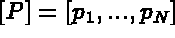
Before writing equation (1.3) in terms of the finite element approximations, let us define the following notation:
 is the partitioning (mesh) of the domain
  , with T an element in
, so that
, with T an element in
, so that
 where
where  denotes the total number of degrees of freedom.
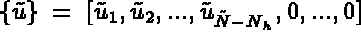
 denotes the values of the global degrees of freedom.
 denotes the values of the local degrees of freedom for element T.
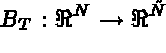
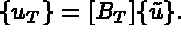
 is the set of degrees of freedom on the boundary.
 (or
(or  ) signifies that the global degree of freedom,
 , belongs to the mesh (or to the boundary).
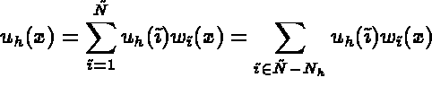
basis functions,
, belongs to the mesh (or to the boundary).
basis functions, 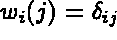 , which spans the subspace ,
then
, which spans the subspace ,
then  , in terms of these basis functions, is given by
 . can be written as
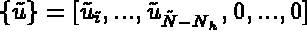
 are the component of on the basis
  , and supposing that the
degrees of freedom on the boundary are numbered last.
, and supposing that the
degrees of freedom on the boundary are numbered last.
 in terms
of the element polynomial basis functions, is given by:
in terms
of the element polynomial basis functions, is given by:
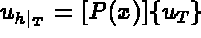 , defined previously.
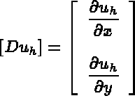
Let the derivative of be defined by
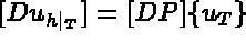
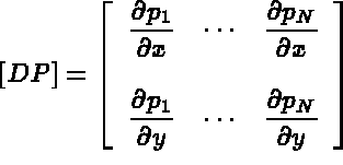
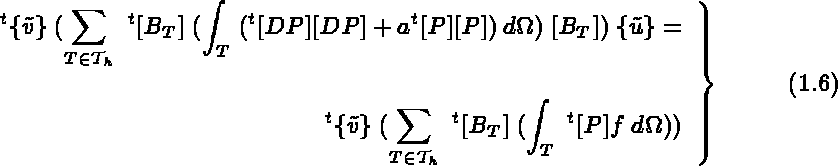
Equation (1.3) in terms of the above finite element notation can now be written as follows:
Find which satisfies
 , for , such that
for any  satisfying
  ,
,  .
.
At this stage, the derivation from formulation (1.3) to formulation (1.6) is quite general (independent of MODULEF). It remains to define the corresponding mathematical operators, after which we must find their equivalents in MODULEF.
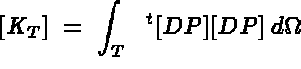
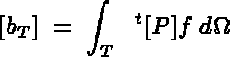
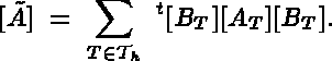
Let us first consider the classical thermal problem, described in [100], which is fully solved by the MODULEF system, where the element stiffness and mass matrices and force vector is given by:
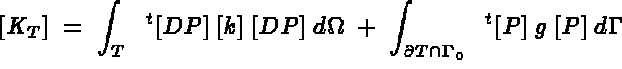
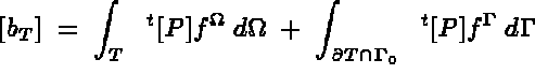
We notice that if we set:
[k] = [I] : the thermal conductivity ([I] : unit matrix),
g=0 : the coefficient of heat transfer at  ,
,
 : the mass density, and
 : the boundary force.
in the classical thermal system, we can define the element stiffness and mass matrices and force vector for the Dirichlet problem in terms of the thermal problem. The resulting simplified system is then given by:
By combining these simplified element calculations, equation (1.6) can now be rewritten, so that our problem can be completely solved by MODULEF, as a thermal type problem.
Remark: A list and the description of the thermal finite elements available in the MODULEF library are given in [100].
In terms of the above notation, (1.6) becomes:
Find which satisfies ,
for , such that
for all  , such that
  , for
, for  , which results in a linear system with a
positive definite symmetric matrix.
, which results in a linear system with a
positive definite symmetric matrix.
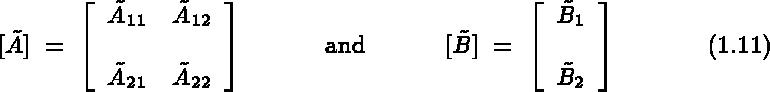
Let  be an element matrix of element T, with corresponding matrix
 .
.
There are two possible interpretations of the above example:
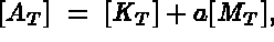
If  is the system matrix to be solved, it may be written as follows:

From a mathematical point of view, these formulas are identical. However, they may lead to two different computer
problems. In both cases it is necessary to calculate the element mass  and stiffness
  matrices,
after which we either:
matrices,
after which we either:
, resulting in [M],
, resulting in [K], and
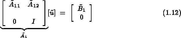
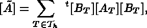
After assembly of the system matrices, equation (1.9) becomes:
Find satisfying , for all , such that
for all satisfying  , for all .
Recall that, for the discrete space  span
span ,
,  is given by:
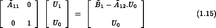
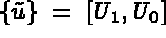
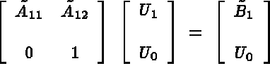
Let us consider the decomposition of and  , such that
where  is a
is a  matrix.
With this decomposition, and by using the properties of and in subspace
into account, equation (1.10) is equivalent to:
Thus, in order to calculate , it is necessary to solve (1.12), or equivalently:
where  is a
is a  -dimensional array,
whose components are the first
-dimensional array,
whose components are the first  components of .
Remarks:
 (equation (1.12)), by assembling the elements
 , necessitates a distinction between the elements for
 and
and  , so that the condition
  is taken into
account.
is taken into
account.
It is therefore simpler to first calculate  and then compute . This operation is
called "imposing the boundary conditions".
and then compute . This operation is
called "imposing the boundary conditions".
The above analysis enables us to extract the different mathematical operators, so that the problem can be decomposed into the following steps:
Remark: Step 1) and 2) result from the chosen variational formulation.
Each step can be decomposed into sub-steps. The decomposition of each step, as well as the choice of modules
which compute the mathematical operators, are briefly discussed in the remainder of this section.
Let us first define the following terminology:
 , lines and points in or ). These numbers allows for the treatment "by block"
of the boundary conditions, the loads, or to define the curved lines (or surfaces).
, lines and points in or ). These numbers allows for the treatment "by block"
of the boundary conditions, the loads, or to define the curved lines (or surfaces).
In the figure 1.1, the body is clamped at boundary AF, and pulled along boundary CD. It is composed of two materials, with a circular hole and a half-circle.
In this configuration there are two sub-domains:
and at least four reference numbers:
Remark: Lines AC and FD do not have reference numbers assigned as no particular conditions applies
there.
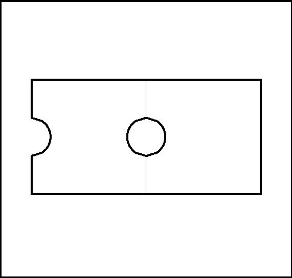
Figure 1.1: Clamped body with applied load
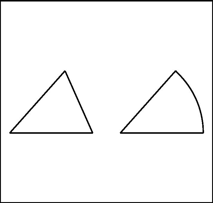
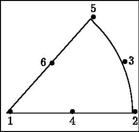
Consider the two elements illustrated in figure 1.2: a straight P2 triangle and a curved P2 triangle. A straight element is an element whose points are the vertices. A curved element is an element whose points are the vertices plus some other characteristics. In the case of a P2 triangle, the straight element is defined by 3, and the curved element by 6 points, both having 6 nodes.
So far we have defined various mathematical operators to solve a typical problem. With each of these mathematical operators we will now associate a computer module, to solve the problem numerically. The data structures (D.S.) provides the interfaces between the modules. In this section we will mention the modules and data structures associated with each step.
This step is the simplest with respect to the mathematical operator. The discretization must respect
the general rules of the finite element mesh. Let  and
and  be elements of then:
|
|
The corresponding implementation is not trivial (see for example [George-1986]) and, even if all the necessary operators are present in the library, it proves labour costly. A well adapted mesh is an essential condition for good results.
The mesh generation technique adopted in MODULEF has a "tree" (top-down, bottom-up) structure, where the domain is partitioned into geometrically simple sub-domains. These sub-domains are then manipulated by simple operators (symmetry, rotation, translation, etc.) and then glued together to obtain the final mesh. This procedure is implemented by the module APNOPO for a two-dimensional domain. The mesh generation technique, as well as the different modules available, are described in detail in [MODULEF User Guide - 3].
The resulting mesh is stored in the D.S. NOPO. This D.S. contains the mesh description: the elements, the nodes (with or without vertices), as well as the coordinates at the vertices, that have been generated.
At this stage the nodes have been numbered. However, the interpolation has not been introduced, which will be discussed in the next step.
Example:
 \
\
A plot of the mesh is generated by module TRNOPO
[4][MODULEF User Guide - 6], which will be discussed in the
next section.
In this step the interpolation of functions are taken into account. This procedure is implemented by module COMACO [13]. Two cases may occur:
The results of this step are found in two data structures: MAIL and COOR. The D.S. MAIL contains the description of the mesh (nodes, points, etc.) and of the interpolation (number and name of the variational unknowns, mnemonics, etc.). The D.S. COOR contains the coordinates of the points (vertices or not).
Note: The D.S. COOR does not contain the coordinates of the nodes on exit from COMACO. Consider again the examples of the elements "straight P2 triangle" and "curved P2 triangle": In the first example the D.S. COOR contains the coordinates of the vertices. In the second example, the D.S. COOR contains the coordinates of the vertices and those of the mid-side points.
The purpose of this step is to construct the element matrices and arrays, , , and  .
This calculation
requires the knowledge of the physical data which describes the materials, loads, temperatures, etc.
In the present example, this corresponds to f and a which appear on the right- and left-hand-side
of the equation. All physical data must be known at the time of activation of the module calculating the
element matrices and arrays.
.
This calculation
requires the knowledge of the physical data which describes the materials, loads, temperatures, etc.
In the present example, this corresponds to f and a which appear on the right- and left-hand-side
of the equation. All physical data must be known at the time of activation of the module calculating the
element matrices and arrays.
There are two possibilities:
In all the cases, it is possible to provide these characteristics by sub-domain and/or reference number, which minimizes the amount of data. The results of this step are found in the D.S. TAE, containing the element matrices and arrays corresponding to all the elements in the mesh.
Remarks:
Other modules implement this step for some specific problems (ex:
[2]
COTAE in nonlinear elasticity with large
deformations [97]; BIHAP1,
[4] BIHAP2 for the biharmonic problem [93], etc.).
This step can be decomposed into several sub-steps. The sub-steps vary according to the desired method of solution, however the basic principles remain the same. The MODULEF library contains a large number of solution methods for linear systems, amongst which are:
In all these cases the matrix corresponding to the finite element discretization, is sparse. In order to minimize the space occupied in memory, an appropriate method of matrix storage is sought:
The non-linear problem can often be solved by regarding it as that of a series of linear problems, each treated as described above.
The choice of solution method for linear systems is not obvious, and depends strongly on the nature of the problem to be solved. In the case of simple systems, all methods produce good results. When there are many systems to solve, for example an iterative process, there are some points in favour of both types of solution methods:
In order to analyze the different sub-steps, consider the simple example of solving a linear system by a direct Cholesky method in main memory (m.m.).
This step is performed by module PREPAC [MODULEF User Guide - 5]. The result is found in the D.S. MUA, which does not contain the matrix but only the pointers.
The results of this step is found in the D.S. MUA, containing the system matrix, and the D.S. B, containing the right-hand-side vector.
The purpose of this step, which consists of two sub-steps, is the implementation of the second type of boundary conditions.
Remark:
to  , considering equations (1.11) and
(1.12).
, considering equations (1.11) and
(1.12).
There are several techniques for implementing boundary conditions, as described in [MODULEF User Guide - 5]: module CLIMPC, for skyline matrices. Conceptually, we can distinguish two classes:
The point of departure is the following "computer" equality:
 (for example:
 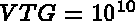 and
and  ).
).
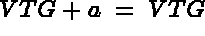
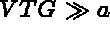
In practice we start with and  of equation (1.11), and replace the
diagonal coefficients of
of equation (1.11), and replace the
diagonal coefficients of  by VTG and the coefficients of
  by
by  , where
where

A variation on the above method consists of replacing the diagonal coefficients of by:
 by:
by:

 .
.
Advantages and disadvantages:
To summarize:
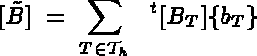
The idea is to derive equation (1.12) from (1.11) effectively. Note that in equation (1.12) an important property, namely the symmetry of the matrix, is lost. The importance lies in the property that for a symmetric matrix only half the matrix needs to be stored. We therefore want to derive (1.15), which is equivalent to equation (1.12), from equation (1.11), where (1.15) is symmetric.
In the general case (imposed d.o.f. has a value of , zero or nonzero (1.14)), if we consider the
decomposition of :

then equation (1.12) can be written as follows:
which is equivalent to:
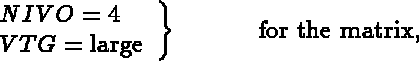
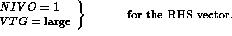
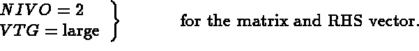
In practice, it is equation (1.15) that is calculated (using the notation in [MODULEF User Guide - 5]:
PROFIL and CLIMPC, with NIVO = 3 and VTG = 1).
Remark: The different techniques above are independent of the matrix storage technique, and can therefore be used in other methods of storage.
The result is stored in the D.S. MUA which contains the factorized matrix.
The result is stored in the D.S. B.
Comments:
The solution of the linear system is decomposed into several steps in order to simplify the computation as
much as possible. For example:
The graphic visualization of results is particularly important. Indeed, it is difficult to interpret the results by merely printing the output data structure B. In order to aid you with the interpretation of results, the following tools are available:
In the post-treatment, we can also utilize the modification modules for the data structures NOPO [MODULEF User Guide - 3] and B. For example, if the problem is symmetric, the computation need only be done on part of the domain. However, it is desirable to present the results on the complete domain, by "gluing" together the sub-domains.
The purpose of this example was to illustrate how find the suitable modules in the libraries, capable of solving the problem under consideration. However, it does not show how to use a given module. The examples treated in the remainder of this report will illustrate this process in detail.