

![[BIG]](../icons/zoom18.gif)
![[Normal]](../icons/zoom14.gif)
![[small]](../icons/zoom10.gif)
Next: 5.2.2 Bottom-up construction
Up: 5.2 A two-dimensional example
Prev: 5.2 A two-dimensional example
Index
Contents

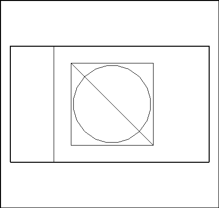
Figure 5.1: The domain under consideration
The domain of interest is shown in figure 5.1. The analysis of the geometry and the presence of
several materials leads us to define four principal parts:
- i
- the shield (part 4.4 of the figure): its quadrilateral form urges us to use the
QUACOO mesh generator, i.e. the algebraic method producing elements of a quadrilateral nature constructed
from the input data consisting of the contour of the part considered;
the data consists of the 4 sides (from a topological point of view);
- ii
- the air zone (part 4.3 of the figure): it corresponds to the quadrilateral pierced by
a square; this implies that the boundary of this part has 2 components; consequently, we will use the
TRIHER mesh generator, i.e. the Voronoi method producing triangular elements constructed from
the input data consisting of the contour of this part; the data consists of the union of the constituent lines;
- iii
- the semiconductor (part 4.2 of the figure): due to its shape, we use, again,
mesh generator TRIHER (Voronoi method) which requires the contour of this part as input data
(i.e the union of the constituent lines);
- iv
- the half-cooling circuit (part 4.1 of the figure): due to its shape, we will again use
mesh generator TRIHER.
The "gluing together" of the meshes of 4.1 and 4.2 (module RECOLC) will result in the mesh of the
corresponding half-square. By symmetry (module
[4] MODNOP), we will obtain the mesh of the symmetric part
of the half-square; by "gluing" it to the preceding mesh
(module RECOLC), the complete mesh of the cooling circuit and its conductor will be constructed.
It remains to "glue" (module RECOLC) this mesh to that of the air zone and then "glue" this
result to the mesh of the shield; finally, the end-result will be stored on file (module SAUVER).
The set of modules necessary is therefore the following:
- to create the meshes: QUACOO and TRIHER;
- to transform the meshes: MODNOP and RECOLC;
- to save the result on file: SAUVER.
In terms of keywords of APNOPO, we have:
- to create the meshes: QUAC and TRIH;
- to transform the meshes: SYMD and RECO;
- to save the result on file: SAUV.
In terms of data, we have successively:
- to create the meshes:
- calling QUACOO, keyword QUAC, requires the data of a discretization of the
contour of the part under consideration. This contour must include 4 sides, amongst them, 2 sides
opposite each other must be described by the same number of sub-segments. An arbitrary side is formed
by one or several characteristic lines. The latter are defined by their 2 end-points and some
parameters describing the manner in which they will be discretized.
- calling TRIHER, keyword TRIH, similarly requires the
data of a discretization of the contour of the part under consideration.
A contour consists of several characteristic lines described as above. In the event that the contour consists
of 2 parts, we input first the external part (in an anti-clockwise direction) followed by the
internal part (in the reverse direction).
- to transform meshes:
- calling MODNOP, keyword SYMD, requires the input of the equation of the line of
symmetry.
- calling RECOLC, keyword RECO, requires the data of parameter
 ,
the precision threshold for the identification of the "gluing" zones.
- to save the result on file:
- calling SAUVER, keyword SAUV, requires the definition of the level of the mesh which
we want to save on file.
In terms of keywords of APNOPO we therefore need, in addition:
- for the creation of the contours: the definition of the lines via LIGN;
- if a line is defined via a curve whose equation is known, it is described using keyword
COUR
- for the creation of the lines: the definition of the points via POIN;


![[BIG]](../icons/zoom18.gif)
![[Normal]](../icons/zoom14.gif)
![[small]](../icons/zoom10.gif)
Next: 5.2.2 Bottom-up construction
Up: 5.2 A two-dimensional example
Prev: 5.2 A two-dimensional example
Index
Contents
![]()
![]()
![]()
![]()
![]()
![]()
![]()
![]()
![]()

 ,
the precision threshold for the identification of the "gluing" zones.