Next: 2 Visualization of meshes Up: Part II: Graphics Prev: Quick guide Contents

1 General structure

In general, the organization of the plotting modules of the MODULEF library can be schematized as follows:

 
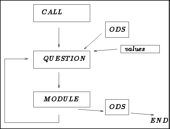
Figure 1.1: General organization of the plotting modules 

• From a practical point of view, a visualization is performed by executing preprocessor "CALL" (see figure 1.1) which calls program "QUESTION".

• This program then requests the user to choose the output device and to indicate the file name(s) containing the data structure(s) ("IDS" in the flowchart) required, or the numerical values ("values" in the flowchart) to plot.

• A general menu or status table is then displayed (in alphanumeric mode), which indicates the visualization parameters, i.e., for each item described, the manner in which it is treated, or the visualization choices available.

• An immediate visualization (the "MODULE" is activated) can also be requested, which corresponds to automatic mode visualization.

• Furthermore, the user can also modify values in the status table until the desired visualization parameters are set before requesting the corresponding visualization.

• Once the plot is displayed, a graphics menu appears on the screen to enable the user to perform certain graphical operations.

The above organization is used for all the graphics modules in the library, except for the surface visualization module, Z=F(X,Y), and the mesh plotting modules utilizing roll-down menus. The following thus applies to all the modules except the two modules, VIS3XX and REFEXX.

 
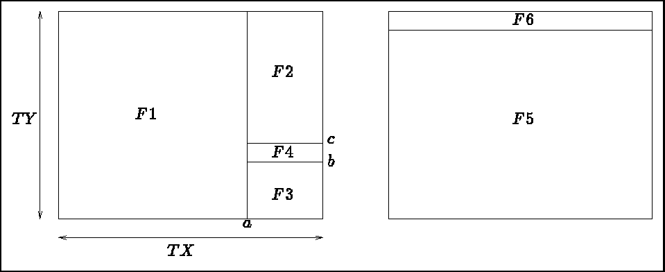
Figure 1.2: Presentation of the screen with and without the general legend 

The plot occupies a box of size on the screen (figure 1.2). This box is split into different zones or windows in which are displayed:

• If a general legend is requested (default option):
  • the object in F1,
  • the general legend in F2.
  • the graphics menu in F3,
  • a quick indication of the type of plot in F4.
• If we request no general legend (key 60 in the general menu, see below):
  • the object in F5,
  • the graphics menu in F6.

The size of the windows is determined as a percentage of the size of the box chosen, which is a function of the device used. The box dimensions are calculated automatically (the entire screen is subdivided), or input by the user (in centimeters).

A mask is associated with each window (measured in centimeters). It is linked to the object visualized above and is consequently measured in the units of this object (mm., cm., ...km., etc.).

When executing a graphics preprocessor, the user must select the output device number, in which case a menu appears. This general menu is presented in the form of a table in which each line has the following form (the line presenting the option whether or not to have a legend is used as an example):

 ------------------------------------------------------------
 | 60 | LEGEND                   |  YES
 ------------------------------------------------------------

 ------------------------------------------------------------
 | KEY | DESCRIPTION of ITEM    |  STATUS of ITEM
 ------------------------------------------------------------

The first column contains a number or key, which must be specified if we want to modify the status (third column) of the item described in column two. There are three kinds of keys:

• the keys which serve as flags: there are only two states possible for the item under consideration (for example, YES or NO, HARD or SOFT, etc.). In this case, the selection of the key has the effect of changing from one state to another. Thus, for key 60 we have:

   ------------------------------------------------------------
   | 60 | LEGEND                   |  YES
   ------------------------------------------------------------
  

  that becomes

   ------------------------------------------------------------
   | 60 | LEGEND                   |  NO
   ------------------------------------------------------------
  

• keys which have multiple choices: there are several states possible for the item under consideration. In this case, the selection of the key results in a choice. Thus, for key 50 we have:

   ------------------------------------------------------------
   | 50 | ITEMS PLOTTED           |         TRIANGULATION
   ------------------------------------------------------------
  

  for which we can choose between:

    -- MESH                                 :
       NOTHING                 : 0
       TRIANGULATION           : 1
       GEOMETRIC CONTOUR       : 2
       REFERENCED BOUNDARY     : 3
       SHRINK                  : 4  ?
  

  Choice 2 (type 2 on the keyboard) then results in the following status:

   ------------------------------------------------------------
   | 50 | ITEMS PLOTTED          |  GEOMETRIC CONTOUR
   ------------------------------------------------------------
  

• keys which display a sub-menu which has the same form as the general menu (a status table with three columns).

Once the status table has the desired configuration (if the user does not intervene, the default options or automatic mode would be employed), we can start the visualization process. The following lines appear at the end of the menu:

 | .. |    ......                    |    ......
 -- PLOT  : 0 , CURRENT STATUS : VIEW ,    END : END
 --         OR NUMBER OF THE ITEM TO MODIFY  ?

• To obtain a plot, type 0 (this initiates the plot).

• To display the status of the parameters, the user requests to see the status table by typing VOIR.

• To end the session, type FIN.

• To modify a value in the menu, type the key (the number) of the line to modify as indicated above (see also, for each module, the nature of the accessible items).

A context of observation (mask, ...) is associated with each plot displayed. This context is placed in a stack. It corresponds to a cyclic list of length 5 which, initialized to 5 times the initial context, will contain the 5 last visualization contexts. The user can position him/herself in the stack as demonstrated below:

When a plot is displayed (window 1 or 5 depending on the existence or not of the general legend, see figure 1.2), there is a graphics menu at our disposal (window 3 or 6). This graphics menu is use to manipulate the plot by offering the following possibilities (variables as a function of the plot type):

• Exit: 0
• Continue: 1
• Next view: 2
• Previous view: 3
• Refresh: 4
• Zoom : 5 M
• Zoom - : 6
• ......
• Soft copy, hard copy: 8 9

This menu works in the following manner: place the cursor in the window where the object under consideration is plotted and validate the position of the cursor by typing the character associated with the choice made (for example, 5 to zoom). There are two types of actions:

1. The cursor position is not important (even though it is necessary to place it in the plot window). This is the case of choice 0.
2. The cursor position is used to define the operation desired. This is the case of choice 5 which corresponds to a zoom. The cursor is used to obtain the extrema of the zoom zone.

The signification of the actions possibles (and their initiation) is the following:

Exit:

to exit from the session: place the cursor on the plot and type 0.

Continue:

to go the the general menu in order to modify a parameter: place the cursor on the plot and type 1. We are now in the general menu's alphanumeric zone.

Next view:

to go to the stack mentioned above and visualize the next plot: place the cursor on the plot and type 2.

Previous view:

the same, but we go to the previous plot: place the cursor on the plot and type 3.

Refresh:

refreshes the screen: place the cursor on the plot and type 4.

Zoom:

zooms in on part of the displayed plot. Two cases:

• zoom defined graphically: place the cursor on the lower left-hand corner of the zone to zoom and type 5, then place the cursor on the upper right-hand corner and type 5 (or inverse).
• zoom defined manually: place the cursor on the plot and type M. The extrema of the zoom zone must be input.

Zoom -:

to display the plot currently on the screen on only a part of this screen ("inverse" zoom operation): place the cursor on the lower left-hand corner of the zone chosen and type 6, then place the cursor on the upper right-hand corner and type 6 (or the inverse).

Section:

to plot only the part of the object (3D) contained within two parallel planes with sides given. Type 6 and input the 2 sides desired.

R L T B + -:

to move (in 3D) the observation point to the right (type R), the left (type L) (the observer turns 20 degrees), by ascending (type T), by descending (type B) (we also turn 20 degrees), by approaching (type +) or departing (type -) (the distance between the point viewed and the point of observation is divided or multiplied by 2.). To obtain the desired effect, place the cursor on the plot and type the appropriate character.

Softcopy:

sends the plot to another device (the plot is reinterpreted as a function of the terminal's possibilities): place the cursor on the plot and type 8. The program then requests the number of the terminal to which the softcopy is sent.

Hardcopy:

sends the screen image to another device: place the cursor on the plot and type 9.

Certain modules offer only part of these possibilities, others possess different ones specially adapted to the module. By typing ? on the plot, a list and significance of all the choices possible is displayed on the screen.